Case Study

Classification

DVS Data Processing

Dynamic vision sensor (DVS) is a Silicon Retina device based on neuromorphic engineering that simulates the human retina perception mechanism for information acquisition. DVS fundamentally differs from traditional frame-based sensors. Similar to how the human retina sends impulses to the brain upon receiving light stimuli, DVS asynchronously and independently receives light intensity signals at the pixel level, encoding visual signals into a continuous stream of spatiotemporal events. Neuromorphic vision sensors lack the concept of “frames.” When changes occur in the real-world scene, neuromorphic vision sensors generate pixel-level outputs (i.e., events). An event specifically includes (t, x, y, p), where x,y are the pixel coordinates in the 2D space, t is the event timestamp, and p is the event polarity. The event polarity represents the brightness change of the scene: increase (positive) or decrease (negative).

DVS Gesture

Network Model

During both the training and inference processes of the DVS gesture data, a loop operation is performed on the time window T. The model structure executed in each loop is as shown in the figure below, where the input is a single frame with a shape of [b,2,40,40]. The final model output is the sum of the outputs of all 60 frames divided by 60.

Figure: DVS-gesture Network Model

This model structure consists of three Conv2dLif modules and two FcLif modules. In the last Fclif module, the output_channel of the Fc layer is 11, which is the number of categories in the DVS gesture model.

Training and Performance

We randomly selected 1176 samples from the dataset for training and 288 samples for validation. We used the Adam optimizer with a learning rate of 1e-2 and weight decay of 1e-4 to train the network. During training, a learning rate fine-tuning strategy was used. Neuron parameters were set to full-sharing mode. After 100 epochs of training, we achieved a top-1 classification accuracy of 94.09% on the validation set.

MNIST-DVS

Network Model

The MNIST-DVS network model consists of three Conv2dLif blocks. Each sample performs a loop operation over time frames, feeding single-frame samples into these three Conv2dLif blocks for feature extraction. A SumLayer follows, aggregating information over the time dimension by adding all time-frame feature maps element-wise and dividing by T, obtaining average information. The model concludes with an FcBlock for classification, containing three fully connected layers. The last Fc layer’s out_channel corresponds to the 10 classification categories.

Figure: MNIST-DVS Network Model

Training and Performance

We trained the network using an SGD optimizer with a learning rate of 1e-1, weight decay of 1e-4, and momentum of 0.9. A learning rate fine-tuning strategy was employed during training. Neuron parameters were in full-sharing mode. After 20 epochs of training, we achieved a top-1 classification accuracy of 99.54% on the validation set.

CIFAR10-DVS

Model Introduction

Figure: CIFAR10-DVS Network Model

Compared to MNIST-DVS, the feature extraction part Conv2dLIf was increased from three to five, while the FcBlock following the SumLayer contains only two Fc layers.

Training and Performance

We used the Adam optimizer with a learning rate of 1e-2 and weight decay of 1e-4 to train the network. A learning rate fine-tuning strategy was applied during training. Neuron parameters were in full-sharing mode. After 100 epochs of training, the top-1 classification accuracy reached 68.23% on the validation set.

Short Video Processing

RGB-gesture

Training and Performance

The model structure for RGB gesture data is consistent with that of DVS gesture. We trained the network using the Adam optimizer with a learning rate of 1e-3 and weight decay of 1e-4, using the model file trained on DVS gesture as a pre-trained model. After 50 epochs of training, we achieved a top-1 classification accuracy of 97.05% on the validation set.

Jester

Network Model

The model used to train the Jester dataset adopts a ResNet18-like structure, as shown below.

Figure: Jester Dataset Training Model

Similar to other models, operations before the SumLayer are performed on single time steps. In the SumLayer layer, results from all time steps are summed and divided by 16, aggregating information over the time dimension. Finally, an Fc layer is used for classification output.

Training and Performance

Training employed an SGD optimizer with a learning rate of 1e-1, weight decay of 1e-4, and momentum of 0.9. A cosine annealing learning rate fine-tuning strategy was used during training. After 200 epochs, a top-1 classification accuracy of 93.87% was achieved on the validation set.

Text Processing

IMDB

Network Model

The IMDB model also performs loop operations over time frames, inputting single-frame information into the model each time. The model first uses an Embedding layer for dimensionality reduction, followed by an FcLif layer for upsampling, and finally through an Fc layer for classification output. The model lacks a time aggregation layer, using the last frame’s result as output.

Figure: IMDB Network Model

Training and Performance

We used the Adam optimizer with a learning rate of 1e-3 and weight decay of 1e-4 for training, fine-tuning the learning rate based on epochs. After 50 epochs of training, we achieved a classification accuracy of 82.8% on the validation set.

Medical Image Processing

LUNA16Cls

Network Model

The Luna16Cls classification task network model comprises three Conv2dLif blocks. Each sample performs a loop operation for time frames, with single-frame samples sent to these blocks for feature extraction. A SumLayer follows to aggregate information over the time dimension, averaging feature maps across frames. The model concludes with an FcBlock for classification, comprising three fully connected layers, with the last layer’s Fc out_channel corresponding to two classification categories.

Figure: Luna16Cls Network Model

Training and Performance

We used an SGD optimizer with a learning rate of 0.05, weight decay of 1e-4, and momentum of 0.9 to train the dataset, employing a learning rate fine-tuning strategy during training. Neuron parameters were in full-sharing mode. After 20 epochs, a top-1 classification accuracy of 90.50% was reached on the validation set, with an inference speed of 72.3 fps on GPU.

Large Scale Event Classification

ESImagenet

Network Model

The backbone network is resnetlif-18, similar to that of the Jester dataset, with LIF neuron mode set to analog, differing from the spike mode used in Jester.

Training and Performance

We used an SGD optimizer with a learning rate of 0.03, weight decay of 1e-4, and momentum of 0.9 for training, employing a learning rate fine-tuning strategy. Neuron parameters were in full-sharing mode. After 25 epochs of training, the top-1 classification accuracy reached 44.16% on the validation set, with an inference speed of 121.6 fps on GPU.

Large Scale Image Classification

Spike-driven Transformer V2

introduction

Spikerformer v2 (Spike driven transformer V2) is a general SNN (Spiking Neural Network) architecture based on Transformer, named “Meta-SpikeFormer”, aiming to provide an energy-efficient, high-performance and universal solution for neuromorphic computing. It can serve as the structure of visual backbone network and performs excellently in visual tasks. Its features are as follows:

1. Low power consumption: It supports the spike-driven paradigm with only sparse addition existing in the network.

2. Universality: It can handle various visual tasks.

3. High performance: It shows an overwhelming performance advantage compared with CNN-based SNNs.

4. Meta-architecture: It provides inspiration for the design of future next-generation Transformer-based neuromorphic chips.

It adopts the Meta-SpikeFormer architecture, drawing on the general visual Transformer architecture. It expands the four convolutional encoding layers in the Spike-driven Transformer into four Conv-based SNN blocks, and adopts pyramid-structured Transformer-based SNN blocks in the last two stages. For specific model introduction, please refer to the original paper [1].

Figure: Network structure diagram of Spike driven transformer V2

performance

This network has achieved relatively excellent accuracy results. In image classification (ImageNet-1K dataset), Meta-SpikeFormer has obtained remarkable achievements. For example, when the number of parameters is 55M, the accuracy can reach 80.0% by adopting the distillation strategy. Under different model scales, compared with other methods, it shows advantages in terms of accuracy, parameters and power consumption. In addition, it has also achieved good accuracy results in various tasks such as event-based action recognition tasks (HAR-DVS dataset), object detection (COCO benchmark), and semantic segmentation (ADE20K and VOC2012 datasets).

Lynxi system deployment

This network model can be deployed through a single KA200 chip. Currently, the default deployed model is the metaspikformer_8_512 model (pretrained weights, 55M parameter version, T = 4 (4 time steps)). The original code model was designed for the Spikingjelly framework. In this case, certain modifications have been made to it and it has been incorporated into this software stack. This code only supports inference and does not support training. If training is required, it is recommended to use the original code framework. Note: This case only guarantees the correct inference results reproduced on the Lingsi brain-like computing chips, and does not guarantee the reproduction of indicators such as power consumption and energy efficiency in the original paper.

References

Original code link: BICLab/Spike-Driven-Transformer-V2

[1]. Yao, Man, et al. “Spike-driven transformer v2: Meta spiking neural network architecture inspiring the design of next-generation neuromorphic chips.” arXiv preprint arXiv:2404.03663 (2024).

Brain-inspired Tracking (Continuous Attractor)

Tiger1 Dataset Object Tracking

Data and Preprocessing

The Tiger1 dataset consists of a video with a resolution of 640×480, totaling 354 frames. Each frame is manually annotated with a bounding rectangle (x, y, w, h) as the groundtruth of the tracking target, where x and y are the coordinates of the top-left corner of the rectangle, and w and h are the width and height of the rectangle, respectively. In the video, there are variations in illumination, occlusion of the target, target deformation, motion blur, and both in-plane and out-of-plane target rotations.

To save graphical memory, we first convert each frame of the color image to a grayscale image and then down-sample it to a 30×56 resolution.

Network Model

The network model used in this task is the Continuous Attractor Neural Network (CANN), a model inspired by neuroscience. As shown in the figure below, x represents coordinates on a two-dimensional plane, and \(V(x,\ t)\)is the membrane potential of a neuron at position x and time t.

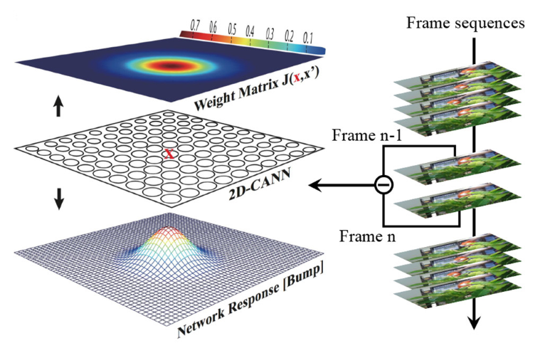
Figure: Original Dynamic Model of CANN Schematic

Example of Object Tracking Based on CANN

, r(x,t) is the firing rate of the neuron. It is reasonable to assume that \(r(x,\ t)\)increases with \(V(x,\ t)\), but saturates under global inhibition. Such a model can be represented as:

\[\begin{array}{r} r(x,t) = \frac{V^{2}(x,t)}{1 + k\int_{- \infty}^{+ \infty} V^{2}\left( x',t \right) dx'}\#(1) \end{array}\]

where \(k\)is a small positive hyperparameter that controls the strength of the global inhibition.

In the CANN model, \(V(x,\ t)\)is determined by external stimuli and recurrent inputs from other neurons as well as its own relaxation. Denoting \(V_{ext}(x,t)\)as the external stimulus to neuron x at time t, the model can be represented as:

\[\begin{array}{r} \tau\frac{\partial V(x,t)}{\partial t} = - V(x,t) + \beta\int_{- \infty}^{+ \infty} J\left( x,x' \right)r\left( x',t \right) dx' + V_{ext}(x,t)\#(2) \end{array}\]

where \(\tau\)is a time constant typically on the order of 1 millisecond, and \(\beta\)determines the proportion between recurrent input and external stimuli. \(J\left( x,x^{'} \right)\)is the interaction (synaptic weight) between the neuron at position \(x^{'}\)and the neuron at position \(x\). \(J\left( x,x^{'} \right)\)is calculated as follows:

\[\begin{array}{r} J\left( x,x^{'} \right) = \frac{J_{0}}{2\pi a^{2}}e^{- \frac{\left| x - x^{'} \right|^{2}}{2a^{2}}} \end{array}\]

where \(J_{0}\)is a constant, \(a\)represents the Gaussian interaction range, \(|x - x^{'}|\)denotes the distance between neurons \(x\)and \(x^{'}\)\(\frac{J_{0}}{2\pi a^{2}}\)is the maximum interaction range. The above formula encodes the synaptic pattern (bump shape) with translational invariance, resulting in similar bump patterns represented by high firing rates of neurons. The response bump can predict the location of the object. Additionally, the neuron distance is circular, meaning the topmost and bottommost neurons and those on the far left and right are connected as neighboring neurons. This symmetry ensures stability of the bumps at the boundaries.

As shown in Figure: Original Dynamic Model of CANN Schematic, the differential signals of every two adjacent frames from the video are injected into the network as external stimuli \(V_{ext}(x,t)\). Each neuron receives the intensity of the corresponding pixel in the 2D differential frame. CANN can smoothly track an object since continuous neural dynamics result in smooth trajectories of response bumps. The trajectories have the following features:

• In the absence of external stimuli, the network can maintain a stationary response bump through recurrent inputs;

• When an object is present, especially a moving one, the network can smoothly alter its response bump according to the moving target. The above video shows an example of object tracking based on CANN, where the red bounding box is the gold standard of the object’s position, and the yellow bounding box reflects the predicted position based on the response bump.

Since long-range connections typically have minimal impact on the neuron’s membrane potential and firing rate, and for easier digital circuit implementation, [Equation#2] can be expressed with minimal accuracy loss as:

\[\begin{split}\begin{array}{r} J\left( x,x^{'} \right) = \left\{ \begin{array}{r} \frac{J_{0}}{2\pi a^{2}}e^{- \frac{\left| x - x^{'} \right|^{2}}{2a^{2}}},\ if\ neuron\ x^{'} \in CF(x,\ R) \\ 0,\ otherwise \end{array} \right.\ \end{array}\end{split}\]

where \(x^{'} \in CF(x,\ R)\)indicates that each neuron x only has local connections with neighboring neurons within an R×R rectangular area centered on x.

Because digital circuits cannot directly support the continuous differential dynamics in [Equation#1] and [Equation#2], an iterative state update method can be used to discretize the continuous dynamics into equivalent differential equations. By setting τ=1 and ∂t=1, the continuous state update of the CANN can be modified into an iterative version.

\[\begin{split}\begin{array}{r} \left\{ \begin{array}{r} V(x,t + 1) = \beta\sum_{x^{'} \in CF}^{}{J\left( x,x^{'} \right)r\left( x^{'},t \right)} + V_{ext}(x,t) \\ r(x,t + 1) = \frac{V^{2}(x,t + 1)}{k\sum_{x^{'}}^{}{V^{2}\left( x^{'},t + 1 \right)}} \end{array} \right.\ \#(3) \end{array}\end{split}\]

Thus, the entire computational data flow becomes \(\{ r(x,\ t)\ \&\ Vext(x,\ t)\}\ \Rightarrow \ V(x,\ t\ + \ 1)\ \Rightarrow \ r(x,\ t\ + \ 1)\ \Rightarrow \ ...\). Through this discretization process, the planar continuous attractor model can be implemented on digital circuits via iteration.

For a better understanding of mapping the CANN topology onto multi-core NN architectures, each iteration of the differential equation (Equation#3) is decomposed into the following 5 steps:

Recurrent Input:

\[V_{1}(x,t + 1) = \beta\sum_{x^{'} \in CF}^{}{J\left( x,x^{'} \right)r\left( x^{'},t \right)}\]

1. Membrane potential:

   \[V(x,t + 1) = V_{1}(x,t + 1) + V_{ext}(x,t)\]

2. Potential square:

   \[V^{2}(x,t + 1) = V(x,t + 1) \cdot V(x,t + 1)\]

3. Inhibition factor:

   \[s_{inh}(t + 1) = \frac{1}{k\sum_{x^{'}}^{}{V^{2}\left( x^{'},t + 1 \right)}}\]

4. Firing rate:

   \[r(x,t + 1) = V^{2}(x,t + 1) \cdot s_{inh}(t + 1)\]

DVS High-speed Target Detection

ST-YOLO Pedestrian Vehicle Detection

Data and Preprocessing

The Gen1 dataset is recorded using a PROPHESEE GEN1 sensor mounted on a car dashboard, with a resolution of \(304 \times 240\)pixels. Labels are generated by using the gray level estimation function of an ATIS camera to create standard gray images at specific frequencies, which are then manually annotated. The dataset contains 39 hours of open road and various driving scenes, including urban, highway, suburban, and rural scenarios. Manually annotated bounding boxes contain two categories: pedestrians and cars.

To facilitate the training of deep learning methods, we cut the continuous shooting data into 60-second segments. In total, 2359 samples were obtained: 1460 training samples, 470 test samples, and 429 validation samples. Each sample is provided in a binary .dat format, where event coding uses 4 bytes to represent the timestamp and 4 bytes for position and polarity. More specifically, the x position uses 14 bits, the y position uses 14 bits, and the polarity uses 1 bit.

Bounding box annotations are provided in numpy format. Each numpy array contains the following fields:

• -ts, timestamp of the box (in microseconds);

• -x, x-coordinate of the top-left corner (in pixels);

• -y, y-coordinate of the top-left corner (in pixels);

• -w, width of the box (in pixels);

• -h, height of the box (in pixels);

• -class id, category of the object: - car is 0; - pedestrian is 1.

The preprocessing step first creates a four-dimensional tensor E:

• The first dimension consists of two components representing polarity;

• The second dimension has T components and is related to T discretization steps in time;

• The third and fourth dimensions represent the height and width of the event camera, respectively.

Events within the time interval [\(t_{a}\), \(t_{b}\)] are processed in the following way for the set E:

\[E(p,\ \tau,\ x,\ y) = \sum_{e_{k} \in \varepsilon}^{}{\delta\left( p\ - \ p_{k} \right)\delta\left( x\ - \ x_{k},\ y\ - \ y_{k} \right)\delta\left( \tau\ - \ \tau_{k} \right)},\ {\ \ \ \ \ \ \tau}_{k} = \left\lfloor \frac{t_{k}\ - \ t_{a}}{t_{b}\ - \ t_{a}} \cdot T \right\rfloor\]

In other words, we create T two-channel frames, where each pixel contains the number of positive and negative events within one of the T time frames. Finally, we flatten the polarity and time dimensions to obtain a three-dimensional tensor of shape (2T, H, W), which is directly compatible with 2D convolutions.

Network Model

The ST-YOLO network can perform target detection on event stream data based on spatiotemporal dynamics. After sequentially inputting the event stream information into the network, it is first processed into tensors representing spatial and temporal events. A new event tensor is input into the network at each time step. Additionally, specific Lif layers will accept the state from the previous time step. The output of the Lif layer after passing through the backbone is used as input for the detection framework. The specific structure is shown in the figure below.

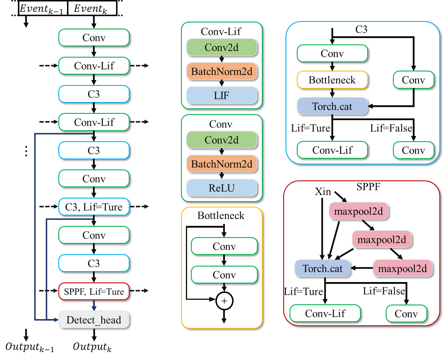
Figure: ST-YOLO Network Architecture Diagram

The network consists of two parts: the backbone and the Detect_head. The backbone part is modified based on the yolov5 backbone, mainly replacing ReLU layers with Lif layers to process time dimension information using the spatiotemporal characteristics of the Lif layer. The Detect_head includes an FPN network and a YoloXhead.

Demonstration

When the GEN1 dataset’s test set is input into the aforementioned network, it can output a sequence of target detection frames from the event stream data. The following video is a demonstration example:

ST-YOLO pedestrian vehicle detection demo

DVS High-Speed Turntable Object Detection with ST-Yolo

Data and Preprocessing

This dataset was collected using Lynxi proprietary high-speed moving target data acquisition device, as depicted in the following figure. After collecting the DVS event stream data, it undergoes processes such as event stream framing, label generation, and dataset integration to form a complete DVS high-speed rotary target detection dataset. The dataset contains three types of targets: {0: ‘Cross’, 1: ‘Triangle’, 2: ‘Circle’}.

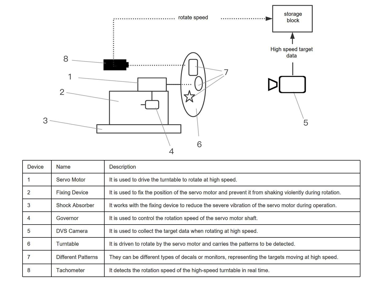
Figure: High-speed moving target data acquisition device

Network Model

The dvs_high-speed_rotary_target_detection utilizes the ST-YOLO network, based on spatiotemporal dynamics, for event stream data target detection. Unlike ST-YOLO Pedestrian Vehicle Detection for vehicle and pedestrian detection, the network head part in this task adopts the yolov5 head due to differences in dataset annotation formats.

Demonstration

The data from the test set is fed into the above network to output a sequence of high-speed turntable event stream data target detection frames. the following video shows a demonstration example:

Location Recognition

Location Recognition Robot Introduction

This quadruped robot is equipped with multiple sensors: an IMU inertial measurement unit for obtaining positional information, an RGB camera for capturing image data, and an event camera for capturing event data; a neuromorphic chip for processing multimodal data.

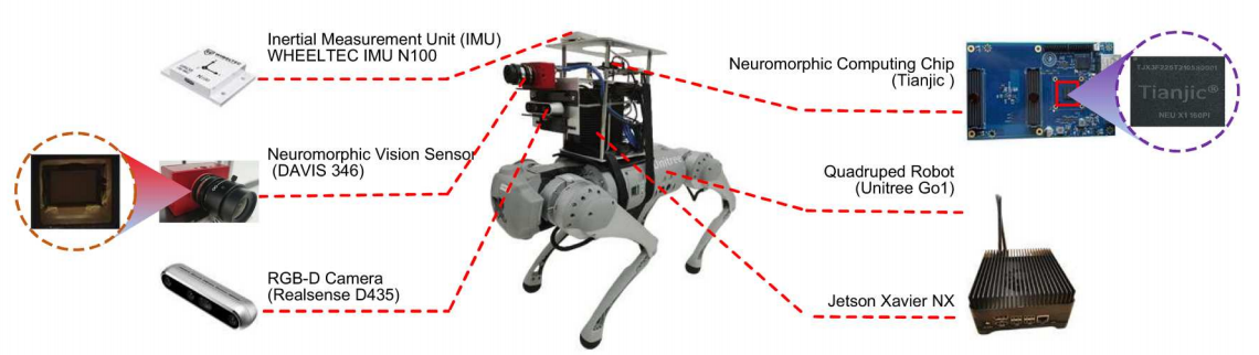
Figure: Location Recognition Robot

Network Model

The architecture of the location recognition network is shown in the figure below. The network consists of four modules: a convolutional neural network (which can use pre-trained ResNet50 or MobileNet_V2) for processing image data, an SNN network for processing event data, a Continuous Attract子 Network (CANN) for processing GPS information, and the multimodal data processed by these three modules is input into the MLSM module (Liquid State Machine) for processing, ultimately obtaining positional information.

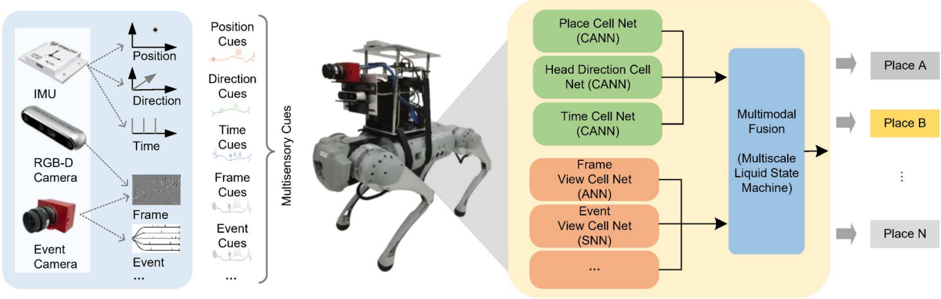
Figure: Location Recognition Network Architecture

Small Target Segmentation and Detection with PCNN

PCNN

The Pulse-Coupled Neural Network (PCNN) is an algorithm inspired by neurobiology, designed mainly for image processing fields such as image segmentation, target recognition, and texture analysis. PCNN simulates the neuron activity in the biological visual system, particularly how neurons in the retina respond to visual stimuli by synchronously firing pulses.

Network Model

The model processes the input image based on PCNN (Pulse-Coupled Neural Network), achieving background suppression and target enhancement. It is used for the detection task of infrared moving small targets.

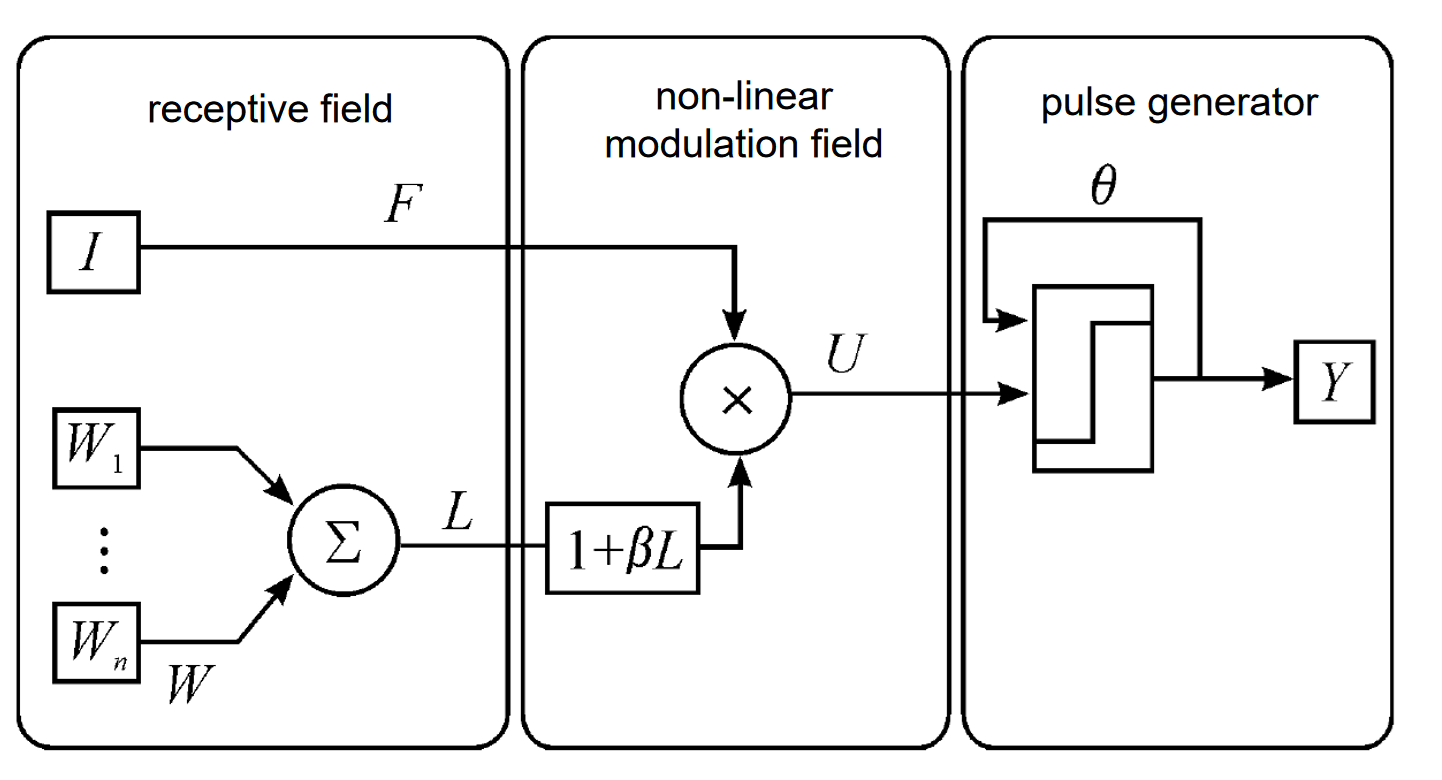
Figure: PCNN network model

Training and Performance

The PCNN network does not require training. The following video shows the detection effect of the PCNN network deployed on the APU.

PCNN network deployed on APU detection effect

PCNN Detection

This case demonstrates the detection of small visible targets (airplanes) based on an improved PCNN. The algorithm requires no complex training and can be used for small sample target detection.

The PCNN network in this case consists of lateral inhibition filters and dynamic neurons with variable thresholds. The first part uses lateral inhibition for image filtering preprocessing to suppress complex backgrounds. The second part uses variable thresholds to generate pulse signals for separating targets from backgrounds. Separation is achieved through pulse firing, with firing neurons representing the target foreground and non-firing representing the background. This process continues for N iterations. During the iteration, the threshold dynamically changes, and through convolution operations, gradually raises the pixel values around firing targets, thereby expanding the target area. Finally, the target area is obtained, and the target area’s position and boundary are calculated for detection output. The adjustment rule for the firing threshold of pixels is as follows: the threshold T varies for each pixel. When the input image pixel is detected as a foreground pixel, T takes the higher value Tmax. When an input pixel does not reach the threshold, T decreases by a fixed amount, making it easier to fire in the next round. The signal O adds itself to X over multiple iterations, collecting all fired neurons to obtain the foreground target. Post-processing further binarizes O and calculates the target box position. The overall process is shown in the figure below.

Figure:pcnn_det algorithm flowchart

The input for detection is a video, and the effect is shown in the video below.

pcnn_det algorithm detection effect example

Frequency/Time/Population Coding

Frequency Encoding

Frequency encoding employs input features to determine the frequency of spikes. The frequency of spikes emitted by a neuron contains all the information. The measure of spike frequency can be completed simply by counting the number of spikes in a time interval, which is the temporal average. The frequency of neuronal spike emission can be understood as the ratio of the average number of spikes observed within a specific time interval T to the time T.

Temporal Encoding

Temporal encoding captures the precise spike timing information of neurons; a single spike carries more meaning than frequency codes that rely on emission frequency. Any spike sequence has a corresponding temporal firing pattern, hence the information related to stimuli might be expressed via the precise spike timing. Specifically, temporal encoding considers that the temporal structure of neuronal spike sequences carries stimulus signals on millisecond or even smaller scales, rather than merely the average firing frequency.

Spike delay coding is a type of temporal encoding, where the method encodes information within the precise spike timing structures of a set of interrelated spikes.

Population Encoding

Distinct from methods that encode through a single neuron, neural information can also be encoded through the activity of multiple neurons. Population encoding is a method of encoding stimulus signals using the collective response of a cluster of neurons. In population encoding, each neuron has a unique spike response distribution to a given input stimulus, with the combined response of neuron groups representing the overall information input.

In this case, population encoding is achieved using a Gaussian tuning curve to convert an analog quantity into a set of spike times for different neurons. A neuron covers a certain range of the analog quantity in the form of a Gaussian function, and the height of the Gaussian function corresponding to a certain value of the analog quantity determines the spike timing of the neuron.

Dataset and Network Model

In this case, the MNIST dataset is encoded and converted into multi-shot spike data as model input. The model adopts

a sequential model of the DVS-MNIST dataset, containing ConvLif x3, FC x3.

Inner Loop SNN

Model Description

The configuration file for the CIFAR10-DVS inner loop case is resnetlif50-it-b16x1-cifar10dvs.py, which uses the ResNet50 model structure, consistent with the outer loop model structure. The model backbone is named ResNetLif, and it is defined in the bidlcls/models/backbones/residual/bidl_resnetlif.py file.

Unlike the outer loop, regardless of running on an APU, the model accepts 5-dimensional data input [t,b,c,h,w]. For the Lif layer, the time axis is unfolded for computation, while for convolution layers and others, the time and batch dimensions are merged to be processed as 4-dimensional data.

Compilation and Deployment

When compiling on an APU, the Lif layer in the model structure needs to use the Lif2dIt class from the bidlcls/models/layers/lif_itin.py file.

Summary of Used Networks in Above Cases

Models in Outer Loop Mode

Simple Sequential

Model	Description
SeqClif3Fc3DmItout	Sequential model for DVS-MNIST dataset, includes ConvLif x3, FC x3;
SeqClif5Fc2DmItout	Sequential model for DVS-MNIST dataset, includes ConvLif x5, FC x2;
SeqClif3Flif2DgItout	Sequential model for DVS-Gesture dataset, includes ConvLif x3, FcLif x2;
SeqClif7Fc1DgItout	Sequential model for DVS-Gesture dataset, includes ConvLif x7, FC x1;
SeqClif5Fc2CdItout	Sequential model for CIFAR10-DVS dataset, includes ConvLif x5, FC x2;
SeqClif7Fc1CdItout	Sequential model for CIFAR10-DVS dataset, includes ConvLif x7, FC x1;
FastText	For IMDB dataset;
SeqClif3Fc3LcItout	Sequential model for Luna16Cls dataset, includes ConvLif x3, FC x3;

ResNet Series

Model	Description
ResNetLifItout-18	Dataset agnostic, ReLU replaced by Lif, includes four stages, each with 2 residual blocks;
ResNetLifItout-50	Dataset agnostic, ReLU replaced by Lif, includes four stages with residual blocks 3, 4, 6, and 3;

Models in Inner Loop Mode

Simple Sequential

Model	Description
SeqClif5Fc2DmIt	Sequential model for DVS-MNIST dataset, includes ConvLif x5, FC x2;
SeqClif7Fc1DgIt	Sequential model for DVS-Gesture dataset, includes ConvLif x7, FC x1;
SeqClif5Fc2CdIt	Sequential model for CIFAR10-DVS dataset, includes ConvLif x5, FC x2;
SeqClif7Fc1CdIt	Sequential model for CIFAR10-DVS dataset, includes ConvLif x7, FC x1;