Designing flow#
The usage flow of BIDL is divided into the following steps:
Construction and Network Training Phase:
Choose or construct a dataset;
Choose or construct a network structure;
Modify the config file and training script;
Network training process;
Use GPU for validation and inference;
Deployment Phase:
Compile the network using Lyngor;
Implement network inference using LynSDK.
Training Part#
Operation Flow#
The main operation flow of the training part is shown in the figure below.

Figure: Training flow#
Add a custom dataset.
Add custom modules.
Add a new backbone network.
Add other components, including new neck, head, and loss function components.
Write configuration files.
Execute GPU training.
Check training results.
Choose or Construct a Dataset#
Select Supported Datasets#
Currently, the datasets added to the BIDL framework are defined in the datasets/ directory. Each dataset corresponds to a file, such as the bidl_cifar10dvs.py file, which implements the functionality of adding the CIFAR10-DVS dataset to the BIDL framework. Different files add different datasets to the BIDL framework. For more details on some of these datasets, refer to Supported Datasets.
Choose different datasets based on the dataset names defined in the files within the datasets/ directory. For example, the CIFAR10-DVS dataset is defined with the name CIFAR10DVS in the bidl_cifar10dvs.py file. This name can be written into the configuration file that requires the use of this dataset. Specific methods can refer to the data section in the Writing Configuration Files paragraph.
Construct a New Dataset#
Datasets can be divided into three categories based on their structure: frame sequences, DVS event data, and one-dimensional data. Frame sequence data is generally constructed by extracting frames at fixed intervals from video clips, while DVS event data is constructed by converting event information into frame sequences.
Different types of datasets have different preprocessing methods, but when added to the BIDL framework, a corresponding file must be defined in the datasets/ directory, and a corresponding class must be defined in the file. The specific steps are as follows:
Write a new dataset class that inherits from BaseDataset.
Overload the
load_annotations(self)method to return a list containing all samples. Each sample is a dictionary containing necessary data information, such as img and gt_label.
The steps for adding a dataset to the BIDL framework are introduced below.
Create a bidl_mydataset.py file in the datasets/ directory and create a MyDateset class in this file to load the data.
from bidlcls.datasets.base_dataset import BaseDataset

class MyDateset(BaseDataset):
   CLASSES = ['class0', 'class1', 'class2', 'class3', 'class4', 'class5', 'class6', 'class7', 'class8', 'class9']

def load_annotations(self):
   print(f'loading {self.data_prefix}.pkl...')
   with open(self.data_prefix + '.pkl', 'rb') as f:
      dats, lbls, shape = pk.load(f)
   data_infos = []
   for dat, lbl in zip(dats, lbls):
      info = {
         'img': dat, 'pack': shape, # \``np.unpackbits`\`
         'gt_label': np.array(lbl, dtype='int64')
      }
   data_infos.append(info)
   return data_infos
Add the newly defined dataset class to datasets/__init__.py.
from .bidl_mydataset import MyDateset # Import the dataset class from the newly written dataset .py file

__all__ = [
   ...,
   'MyDateset', # Add the new dataset class
   ...
]
Use the new dataset in the configuration file in the configs/ directory. For detailed usage of the configuration file, refer to the writing configuration file section in Writing Configuration Files.
dataset_type = 'MyDateset' # Name of the new dataset
...
data = dict(
   samples_per_gpu=64,
   workers_per_gpu=2,
   train=dict(
      type=dataset_type,
      data_prefix='./data/mydataset/train', # Path to the new dataset
      pipeline=train_pipeline,
      test_mode=False
   ),
   val=dict(
      type=dataset_type,
      data_prefix='./data/mydataset/test',
      pipeline=test_pipeline,
      test_mode=True
   ),
   test=dict(
      type=dataset_type,
      data_prefix='./data/mydataset/test',
      pipeline=test_pipeline,
      test_mode=True
   )
)
Choose or Construct a Network Model#
Select Existing Network Models#
The existing network models in the BIDL framework are defined in the /backbones directory. The currently supported network models can be referenced in Models in Outer Loop Mode, and can be deployed on Lynxi brain-inspired systems. For VGG7_SNN model ,the VGG7_SNN.py and VGG7_SNNIt.py define outer loop network models, where the time step loop exists outside the neural network layers, differing from models where the time step loop exists within the network layers.
Based on the characteristics of the dataset, such as scale or complexity, different network models can be selected for training. For example, for the Cifar10Dvs dataset, both the SeqClif5Fc2CdItout and ResNetLifItout network models can be selected at applications/classification/dvs/cifar10dvs directory .
The network model selected for a specific dataset needs to have its name written into the configuration file corresponding to the dataset. The specific method can be referenced in the writing model configuration file section in Content of the Configuration Files.
Construct a New Network Model#
The suffix of the typical outer loop network model names is Itout, which is short for Iterate outside, indicating that the time step loop exists outside the neural network layers.
Sequential Class Networks
The process of adding the SeqClif3Fc3DmItout network model, which resembles a VGG-like network, is introduced below as an example of adding a Sequential class outer loop network model to the BIDL framework.
In the file applications/classification/dvs/dvs_mnist/clif3fc3dm/backbone.py, add the SeqClif3Fc3DmItout network model with time loops outside the layers.
In the network construction part, the three convolutional layers of this network use conv2dLif and set use_inner_loop=False , it can only handle a single time step. The results of each time step need to be aggregated together. The mode used here is mean, indicating averaging, although sum or pick modes can also be chosen. The data dimension before the Flatten layer is (B,C,H,W), so the Flatten layer combines the CHW dimensions and then inputs them into the following three fully connected network layers. This three-layer fully connected network can use the nn.Sequential structure to make the code more concise.
In the network forward part, when running on specific network layers for the first time, it is necessary to explicitly call the reset method to assign the shape to some state variables in the layers. Detailed introductions of these network layers can be found in Neuronal Models. Moreover, depending on whether training is on GPU or inference is on Lynxi brain-inspired systems, there are two branches: for the GPU training branch, the execution process is consistent with the sequence in the network construction part, the three convolutional layers are executed for all time steps using a loop, and the results of all time steps are averaged. Then the data is flattened and input into the fully connected network. For the chip inference branch, as the execution process for all time steps is the same, only one execution of the three convolutional layers is needed, then all time step results are added up using ops.custom.tempAdd, then flattened and input into the fully connected network. By tracing, the corresponding op graph can be generated and mapped onto the chip. The LynSDK cyclic call can achieve the time step loop, and for the averaging corresponding to GPU training, the LynSDK will average the results from tempAdd.
class SeqClif3Fc3DmItout(nn.Module):

   def __init__(self,
               timestep=20, input_channels=2, h=40, w=40, nclass=10, cmode='spike', amode='mean', soma_params='all_share',
               noise=0, neuron='lif', neuron_config=None,spike_func=None,use_inner_loop=False):
      super(SeqClif3Fc3DmItout, self).__init__()
      neuron=neuron.lower()
      assert neuron in ['lif']
      self.clif1 = Conv2dLif(input_channels, 32, 3, stride=1, padding=1, mode=cmode, soma_params=soma_params, noise=noise,spike_func=None,use_inner_loop=False)
      self.mp1 = nn.MaxPool2d(2, stride=2)
      self.clif2 = Conv2dLif(32, 64, 3, stride=1, padding=1, mode=cmode, soma_params=soma_params, noise=noise,spike_func=None,use_inner_loop=False)
      self.mp2 = nn.MaxPool2d(2, stride=2)
      self.clif3 = Conv2dLif(64, 128, 3, stride=1, padding=1, mode=cmode, soma_params=soma_params, noise=noise,spike_func=None,use_inner_loop=False)
      self.mp3 = nn.MaxPool2d(2, stride=2)
      assert amode == 'mean'
      self.flat = Flatten(1, -1)
      self.head = nn.Sequential(
            nn.Linear((h // 8) * (w // 8) * 128, 512),
            nn.ReLU(),
            nn.Linear(512, 128),
            nn.ReLU(),
            nn.Linear(128, nclass)
      )
      self.tempAdd = None
      self.timestep = timestep
      self.ON_APU = globals.get_value('ON_APU')
      self.FIT = globals.get_value('FIT')
      self.MULTINET = globals.get_value('MULTINET')
      self.MODE = globals.get_value('MODE')

   def reset(self, xi):
      self.tempAdd = pt.zeros_like(xi)

   def forward(self, xis: pt.Tensor) -> pt.Tensor:
      if self.ON_APU:
            assert len(xis.shape) == 4
            x0 = xis
            x1 = self.mp1(self.clif1(x0))
            x2 = self.mp2(self.clif2(x1))
            x3 = self.mp3(self.clif3(x2))
            x4 = self.flat(x3)
            x5 = self.head(x4)
            x5 = x5.unsqueeze(2).unsqueeze(3)
            self.reset(x5)
            if self.MULTINET:
               self.tempAdd = load_kernel(self.tempAdd, f'tempAdd', uselookup=True, mode=self.MODE,init_zero_use_data=x5)
            else:
               self.tempAdd = load_kernel(self.tempAdd, f'tempAdd', mode=self.MODE,init_zero_use_data=x5)
            self.tempAdd = self.tempAdd + x5 / self.timestep
            output = self.tempAdd.clone()
            if self.MULTINET:
               save_kernel(self.tempAdd, f'tempAdd', uselookup=True, mode=self.MODE)
            else:
               save_kernel(self.tempAdd, f'tempAdd', mode=self.MODE)
            return output.squeeze(-1).squeeze(-1)

      else:
            t = xis.size(1)
            xo = 0
            for i in range(t):
               x0 = xis[:, i, ...]
               if i == 0: self.clif1.reset(x0)
               x1 = self.mp1(self.clif1(x0))
               if i == 0: self.clif2.reset(x1)
               x2 = self.mp2(self.clif2(x1))
               if i == 0: self.clif3.reset(x2)
               x3 = self.mp3(self.clif3(x2))
               x4 = self.flat(x3)
               x5 = self.head(x4)
               xo = xo + x5 / self.timestep
            return xo
Import the custom new backbone network in backbones/__init__.py or applicationsclassification__init__.py.
from .dvs.dvs_mnist.backbone import SeqClif3Fc3DmItout # Import new module class from written new module.py file
...
__all__ = [
   ...,
   'SeqClif3Fc3DmItout' # Add the new module
   ...
]
Use the new backbone network in the configuration files under the corresponding folders for each dataset. Refer to the Writing Configuration Files documentation for detailed usage of configuration files.
model = dict(
...
   backbone=dict(
      type='SeqClif3Fc3DmItout', # Name of the new module
      timestep=20,
      c0=2,
      h0=40,
      w0=40,
      nclass=10,
      cmode='analog',
      amode='mean',
      noise=0
   ),
...
)
Non-Sequential Network
Below is an example of adding a ResNetLifItout network model to introduce the steps for adding non-Sequential class external loop network models in the BIDL framework.
Add the ResNetLifItout network model with the time loop outside the layers in the file backbonesResNet_SNNResNet_SNN.py.
For the network construction part, refer to the classic ResNet build method to construct the network, using global average pooling for the pooling layer.
Due to the complexity of non-Sequential network structures, during the first run of specific network layers, the state variables are not assigned shapes via a manual explicit call to the reset method, but rather through registering custom hooks.
Use the register_forward_pre_hook method provided by nn.modules to traverse all layers of the network in the _register_lyn_reset_hook function, registering a custom lyn_reset_hook for layers where the state variables need to be assigned shapes. In our custom hook, add an attribute lyn_cnt to layers registered with this hook and initialize it to 0. During the first time step of a sample forward, the layer calls its reset method to assign shapes to the state variables and increments its lyn_cnt. At other time steps, since lyn_cnt is not 0, the layer’s reset method is not called.
After all time steps of a sample forward are completed, call the self._reset_lyn_cnt method to reset the lyn_cnt to zero for the next sample to assign shapes to the state variables in specific layers.
On GPU training, execution follows the same order as the network build part, with layers before the fully connected ones executed in a loop for all time steps, then averaging the results of all time steps before inputting to the fully connected network.
# Define BasicBlock class referencing the classic ResNet build method
class BasicBlock(nn.Module):
   pass # Omitted here

# Define BottleNeck class referencing the classic ResNet build method
class Bottleneck(nn.Module):
   pass # Omitted here

# Define ResNetLifItout class
class ResNetLifItout(nn.Module):

   # ResNet depth and corresponding Block structure and quantity
   arch_settings = {
      10: (BasicBlock, (1, 1, 1, 1)),
      18: (BasicBlock, (2, 2, 2, 2)),
      34: (BasicBlock, (3, 4, 6, 3)),
      50: (Bottleneck, (3, 4, 6, 3)),
      101: (Bottleneck, (3, 4, 23, 3)),
      152: (Bottleneck, (3, 8, 36, 3))
   }

   def __init__(
      self,
      depth,
      nclass,
      low_resolut=False,
      timestep=8,
      input_channels=3,
      stem_channels=64,
      base_channels=64,
      down_t=(4, 'max'),
      zero_init_residual=False,
      noise=1e-3,
      cmode='spike',
      amode='mean',
      soma_params='all_share',
      norm =None
   ):

   super(ResNetLifItout, self).__init__()

   # Other special initialization processes
   assert down_t[0] == 1
   ...

   # Generate corresponding layers based on different Block structures referencing classic ResNet implementation method, specifics not covered here
   @staticmethod
   def _make_layer(block, ci, co, blocks, stride, noise, mode='spike', soma_params='all_share', hidden_channels=None):
      pass # Omitted here

   # Register custom self.lyn_reset_hook to all Lif2d layers
   def _register_lyn_reset_hook(self):
      for child in self.modules():
         if isinstance(child, Lif2d): # Lif, Lif1d, Conv2dLif, FcLif...
            assert hasattr(child, 'reset')
            child.register_forward_pre_hook(self.lyn_reset_hook)

   # In this hook, the reset method for specific layers is only called once when their attribute lyn_cnt is 0
   def lyn_reset_hook(m, xi: tuple):
      assert isinstance(xi, tuple) and len(xi) == 1
      xi = xi[0]
      if not hasattr(m, 'lyn_cnt'):
         setattr(m, 'lyn_cnt', 0)
      if m.lyn_cnt == 0:
         # print(m)
         m.reset(xi)
         m.lyn_cnt += 1
      else:
         m.lyn_cnt += 1

   # This method is called after all time steps of a sample are completed
   def _reset_lyn_cnt(self):
      for child in self.modules():
         if hasattr(child, 'lyn_cnt'):
            child.lyn_cnt = 0

   # Rewrite forward method, input is sample, return value is the result of the last fully connected layer of ResNet, specifics not covered here
   def forward(self, x):
      x5s = []
      for t in range(xis.size(1)):
         xi = xis[:, t, ...]
         x0 = self.lif(self.conv(xi))
         x0 = self.pool(x0)
         x1 = self.layer1(x0)
         x2 = self.layer2(x1)
         x3 = self.layer3(x2)
         x4 = self.layer4(x3)
         x5 = self.gap(x4)
         x5s.append(x5)
         xo = (sum(x5s) / len(x5s))[:, :, 0, 0]
         xo = self.fc(xo)
         self._reset_lyn_cnt()
         return xo
Import the custom new backbone network in bidlcls/models/backbones/__init__.py.
from .ResNet_SNN.ResNet_SNN import ResNetLifItout # Import new module class from written new module.py file
...

__all__ = [
   ...,
   'ResNetLifItout', # Add the new module
   ...
]
Use the new backbone network in the configuration files under the corresponding directories for each dataset. Refer to the configuration file writing instruction document for the detailed usage method.
model = dict(
   ...
   backbone = dict(
      type = 'ResNetLifItout',      # Name of the new module
      depth = 10,                   # Configuration information of the new module
      nclass = 11,
      other_args = xxx
   ),
   ...
)
Writing Configuration Files#
All configuration files are placed in the corresponding directory of application. The basic structure of the directory is:
Category of dataset/Name of dataset/Model name used for the dataset/Configuration file
Naming Rules for Configuration Files#
The configuration file name consists of three parts:
Model information
Training information
Data information
Words belonging to different parts are connected by a hyphen -.
Model Information
Refers to the information of the backbone network model, such as:
clif3fc3dm_itout
clif3flif2dg_itout
clif5fc2cd_itout
resnetlif10_itout
itout is an abbreviation for iterate outside, indicating that the time step loop is outside the neural network layer. Typical external loop network model names have an itout suffix.
Training Information
Refers to the settings of the training strategy, including:
Batch size
Number of GPUs
Learning rate strategy, optional
Examples:
b16x4means the batch size per GPU is 16, and the thread count per GPU is 4;cos160emeans using the cosine annealing learning rate strategy with a maximum epoch of 160.
Data Information
Indicates the dataset used, such as:
dvsmnist
cifar10dvs
jester
Example of Configuration File Naming#
resnetlif18-b16x4-jester-cos160e.py
It uses resnetlif18 as the backbone network. The training strategy is that the batch size per GPU is 16, the thread count per GPU is 4, the dataset is the jester dataset, and it adopts the cosine annealing learning rate strategy with a maximum of 160 epochs.
Content of the Configuration Files#
There are 4 basic components in the configuration files:
Model (model)
Data (data)
Training strategy (schedule)
Runtime settings (runtime)
Take applications/classification/dvs/dvs-mnist/clif3fc3dm/clif3fc3dm_itout-b16x1-dvsmnist.py as an example to explain the above four parts respectively.
Model (model)
In the configuration file, the model parameter ‘model’ is a Python dictionary, mainly including network structure, loss function, etc.:
type: Name of the classifier, currently only ImageClassifier is supported;
backbone: Backbone network, optional items refer to the supported model description document;
neck: Neck network type, currently not in use;
head: Head network model;
loss: Type of loss function, supporting CrossEntropyLoss, LabelSmoothLoss, etc.
model = dict(
   type='ImageClassifier',
   backbone=dict(
      type='SeqClif3Fc3DmItout', timestep=20, c0=2, h0=40, w0=40, nclass=10,
      cmode='analog', amode='mean', noise=0, soma_params='all_share',
      neuron='lif',           # neuron mode: 'lif' or 'lifplus'
      neuron_config=None      # neron configs:
                              # 1.'lif': neuron_config=None;
                              # 2.'lifplus': neuron_config=[input_accum, rev_volt, fire_refrac,
                              # spike_init, trig_current, memb_decay], eg.[1,False,0,0,0,0]
      ),
   neck=None,
   head=dict(
      type='ClsHead',
      loss=dict(type='LabelSmoothLoss', label_smooth_val=0.1, loss_weight=1.0),
      topk=(1, 5),
      cal_acc=True
   )
)
Note
Currently, the models of the BIDL framework are mainly integrated into the backbone, with the neck temporarily unused, and the head only specifying the loss function and evaluation metrics of the classification head network.
Data (data)
The model parameter ‘model’ in the configuration file is a Python dictionary, mainly including construction data loader (dataloader) configuration information:
samples_per_gpu: When building the dataloader, the batch size per GPU;
workers_per_gpu: The number of threads per GPU when building the dataloader;
train | val | test: Construct the dataset.
type: Dataset type, supporting ImageNet, Cifar, DVS-Gesture, etc.
data_prefix: Root directory of the dataset.
pipeline: Data processing pipeline.
dataset_type = 'MyDateset' # Dataset name

# Training data processing pipeline
train_pipeline = [
   dict(type='RandomCropVideo', size=40, padding=4),           # Random crop with time axis samples
   dict(type='ToTensorType', keys=['img'], dtype='float32'),   # Convert image to torch.Tensor
   dict(type='ToTensor', keys=['gt_label']),                   # Convert gt_label to torch.Tensor
   dict(type='Collect', keys=['img', 'gt_label'])              # Decide which keys in the data should be passed to the detector, pass img and gt_label during training
]

# Test data processing pipeline
test_pipeline = [
   dict(type='ToTensorType', keys=['img'], dtype='float32'),   # Convert image to torch.Tensor
   dict(type='Collect', keys=['img'])                          # No need to pass gt_label during testing
]
data = dict(
   samples_per_gpu=16,                    # Batch size per GPU
   workers_per_gpu=2,                     # Number of threads per GPU
   train=dict(
      type=dataset_type,                  # Dataset name
      data_prefix='./data/mydataset/train', # Dataset directory file
      pipeline=train_pipeline             # Data processing pipeline required for the dataset
   ),
   val=dict(
      type=dataset_type, # Dataset name
      data_prefix='./data/mydataset/test',   # Dataset directory file
      pipeline=test_pipeline,             # Data processing pipeline required for the dataset
      test_mode=True
   ),
   test=dict(
      type=dataset_type,
      data_prefix='./data/mydataset/test',
      pipeline=test_pipeline,
      test_mode=True
   )
)
The data processing pipeline (pipeline) defines all the steps for preparing the data dictionary, composed of a series of operations, each of which takes a dictionary as input and outputs a dictionary. The methods of operations in the data pipeline are defined in the bidlcls/datasets/pipeline folder.
Operations in the data pipeline can be divided into the following three categories:
Data loading: Load image from the file, defined in pipelines/bidl_loading.py
Preprocessing: Rotate and crop images, defined in pipelines/bidl_formating.py and pipelines/bidl_transform.py, such as
RandomCropVideo()for random cropping on images.Formatting: Convert images or labels to the specified data type, defined in pipelines/bidl_formating.py, such as
ToTensorType()to convert processed images to Tensor type.
Training Strategy (schedule)
It mainly includes optimizer settings, optimizer hook settings, learning rate strategies, and runner settings.
optimizer: Optimizer setting information, supporting all optimizers in PyTorch, with parameter settings consistent with those in PyTorch. Refer to the relevant PyTorch documentation for details.
optimizer_config: Configuration file for optimizer hook, such as setting gradient clipping.
lr_config: Learning rate strategy, supporting CosineAnnealing, Step, etc.
optimizer = dict(
   type='SGD',          # Type of optimizer
   lr=0.1,              # Learning rate of the optimizer
   momentum=0.9,        # Momentum
   weight_decay=0.0001  # Weight decay coefficient
)
optimizer_config = dict(grad_clip=None)               # Most methods do not use gradient clipping (grad_clip)
lr_config = dict(policy='CosineAnnealing', min_lr=0)  # Learning rate adjustment strategy
runner = dict(type='EpochBasedRunner', max_epochs=40) # Type of runner used
Runtime Settings (runtime)
It mainly includes the weight-saving strategy, log configuration, training parameters, breakpoint weight path, and working directory information:
checkpoint_config = dict(interval=1)   # The interval of saving checkpoints is 1, the unit can be epoch or iter depending on the runner
log_config = dict(interval=50,         # The interval of logging
dist_params = dict(backend='nccl')     # Parameters for setting up distributed training, and the port can also be set
log_level = 'INFO'                     # Log output level
load_from = None                       # Restore from the given checkpoint path. The training mode will be restored from the round saved in the checkpoint.
resume_from = None                     # Restore from the given checkpoint path. The training mode will be restored from the round saved in the checkpoint.
Execute GPU Training#
The entry point for training is tools/train.py, and dist_train.sh in the same directory provides single-machine multi-card training.
Prerequisite: The configuration file has been written, including model, data, training strategies, etc. Specific instructions are in Writing Configuration Files.
For example, use the resnetlif10-b16x1-dvsmnist.py configuration file.
Execute the following command in the tools/ directory to start training.
python train.py --config resnetlif10-b16x1-dvsmnist
View Training Logs#
The logs and checkpoints from training are archived in work_dirs/resnetlif10-b16x1-dvsmnist/. For the directory of saved files, refer to Model Training.
Evaluation and Deployment to Lynxi Brain-inspired Chips (APU)#
The deployment section includes evaluation on the GPU initially and then methods to replace the backbone suited to Lyngor compilations. Finally, conducting evaluations/deployments on the APU.
Evaluating with GPU#
Evaluation entry point: tools/test.py
Prerequisites: A configuration file containing necessary details about the model, data, and training strategies should be prepared. For detailed instructions, see Writing Configuration Files.
Set the use_lyngor flag to 0, indicating that GPU is used for compilation.
--use_lyngor 0 # Whether to use Lyngor for compilation, set to 0 for GPU
Set the --config and --checkpoint to select the predefined configuration file and the corresponding checkpoint file.
For example, utilize the latest.pth weight file from the resource package weight_files under the corresponding path to evaluate model performance on the Jester validation set:
Run the following command in the tools/ directory:
python test.py --config resnetlif18-itout-b20x4-16-jester --checkpoint latest.pth --use_lyngor 0 --use_legacy 0
The inference speed and accuracy will be displayed in the terminal.
Compilation and Deployment using Lynxi brain-inspired systems#
Note
This section requires deploying the software package on Lynxi brain-inspired systems (server or embedded box) without GPU support.
To compile and deploy using Lynxi brain-inspired systems, append the parameter --use_lyngor 1 when executing commands.
Compiling with Lyngor#
To compile using Lyngor, additionally append the parameter --use_legacy 0 after executing the command, meaning it will not load historical compiled artifacts but directly compile.
Prerequisites: Using Lyngor for compilation requires executing the build_run_lif.sh script in the lynadapter directory and registering custom operators in Lyngor.
if args.use_lyngor == 1:
   globals.set_value('ON_APU', True)
   globals.set_value('FIT', True)
   if 'soma_params' in cfg.model["backbone"] and cfg.model["backbone"]['soma_params'] == 'channel_share':
      globals.set_value('FIT', False)
else:
   globals.set_value('ON_APU', False)
   cfg.data.samples_per_gpu = 1
In the code above, if it detects APU compilation, it will set the backbone configuration parameters on_apu and fit to True, meaning each LIF class instance will generate a UUID and part of the LIF neuron’s computation will be implemented using custom operators. Additionally, the dataset batchsize is set to 1, and input type is set to uint8 to fit the underlying requirements.
dataset,_ = get_data(data_name, data_set, cfg)
t, c, h, w = dataset.__getitem__(0)['img'].shape
in_size = [((1, c, h, w),)]
input_type=”uint8”
from lynadapter.lyn_compile import model_compile
model_compile(model.eval(),model_file,in_size,args.v,args.b,input_type="float16",post_mode=post_mode, profiler=profiler)
In the code above, the input size, i.e., t,c,h,w values, is obtained from the dataset. Then, the model_compile method from lyn_compilee is used to execute Lyngor compilation with in_size as a four-dimensional size and batchsize set to 1.
In the model_compile method, the main call is to the run_custom_op_in_model_by_lyn() function for compilation operations. This function calls Lyngor-related interface functions to load and compile the model. The specific implementation code is as follows:
def run_custom_op_in_model_by_lyn(in_size, model, dict_data,out_path,target="apu"):
   dict_inshape = {}
   dict_inshape.update({'data':in_size[0]})

   # 1.DLmodel load
   lyn_model = lyn.DLModel()
   model_type = 'Pytorch'
   lyn_model.load(model, model_type, inputs_dict = dict_inshape)

   # 2.DLmodel build
   # lyn_module = lyn.Builder(target=target, is_map=False, cpu_arch='x86', cc="g++")
   lyn_module = lyn.Builder(target=target, is_map=True)
   opt_level = 3
   module_path=lyn_module.build(lyn_model.mod, lyn_model.params, opt_level, out_path=out_path)
Assuming the configuration file is named clif3fc3dm_itout-b16x1-dvsmnis.py, it will generate a folder named Clif3fc3dm_itoutDm in the same directory as the configuration file. The compiled artifacts will be stored in this folder, as detailed below:
.

├── Net_0
│   ├── apu_0
│   │   ├── apu_lib.bin
│   │   ├── apu_x
│   │   │   ├── apu.json
│   │   │   ├── cmd.bin
│   │   │   ├── core.bin
│   │   │   ├── dat.bin
│   │   │   ├── ddr_config.bin
│   │   │   ├── ddr.dat
│   │   │   ├── ddr_lut.bin
│   │   │   ├── lookup_ddr_addr.bin
│   │   │   ├── lyn__2023-12-11-16-28-59-076024.mdl
│   │   │   ├── pi_ddr_config.bin
│   │   │   ├── snn.json
│   │   │   └── super_cmd.bin
│   │   ├── case0
│   │   │   └── net0
│   │   │   └── chip0
│   │   │   └── tv_mem
│   │   │   └── data
│   │   │   ├── input.dat
│   │   │   ├── output.dat
│   │   │   └── output_ddr.dat
│   │   ├── data
│   │   │   └── 100
│   │   │   ├── dat.bin
│   │   │   ├── input.dat
│   │   │   ├── output.dat
│   │   │   ├── output_ddr_2.dat
│   │   │   └── output_ddr.dat
│   │   ├── fpga_config.log
│   │   └── prim_graph.bin
│   └── top_graph.json
└── net_params.json
Skipping Lyngor Compilation#
If there are already compiled artifacts for the relevant model, one can skip the recompilation steps and directly load the historical artifacts. This can be done by adding --use_legacy 1 when running the command.
SDK Inference#
Once the model’s compiled artifacts are available, SDK inference can proceed. First, instantiate the ApuRun class using the chip ID, path to the compiled artifacts, and timestamp.
arun = ApuRun(chip_id, model_path,t)
During instantiation, the self._sdk_initialize() function is called to perform model initialization.
def _sdk_initialize(self):
ret = 0

self.context, ret = sdk.lyn_create_context(self.apu_device)
error_check(ret != 0, "lyn_create_context")

ret = sdk.lyn_set_current_context(self.context)
error_check(ret != 0, "lyn_set_current_context")

ret = sdk.lyn_register_error_handler(error_check_handler)
error_check(ret != 0, "lyn_register_error_handler")

self.apu_stream_s, ret = sdk.lyn_create_stream()
error_check(ret != 0, "lyn_create_stream")

self.apu_stream_r, ret = sdk.lyn_create_stream()
error_check(ret != 0, "lyn_create_stream")

self.mem_reset_event, ret = sdk.lyn_create_event()
error_check(ret != 0, "lyn_create_event")
Then the self._model_parse() function is called for model parameter parsing and memory space allocation.
def _model_parse(self):
   ret = 0
   self.modelDict = {}
   model_desc, ret = sdk.lyn_model_get_desc(self.apu_model)
   error_check(ret != 0, "lyn_model_get_desc")
   self.modelDict['batchsize'] = model_desc.inputTensorAttrArray[0].batchSize
   self.modelDict['inputnum'] = len(model_desc.inputTensorAttrArray)
   inputshapeList = []

   for i in range(self.modelDict['inputnum']):
      inputDims = len(model_desc.inputTensorAttrArray[i].dims)
      inputShape = []

   for j in range(inputDims):
      inputShape.append(model_desc.inputTensorAttrArray[i].dims[j])
      inputshapeList.append(inputShape)
      self.modelDict['inputshape'] = inputshapeList
      self.modelDict['inputdatalen'] = model_desc.inputDataLen
      self.modelDict['inputdatatype'] = model_desc.inputTensorAttrArray[0].dtype
      self.modelDict['outputnum'] = len(model_desc.outputTensorAttrArray)
      outputshapeList = []

   for i in range(self.modelDict['outputnum']):
      outputDims = len(model_desc.outputTensorAttrArray[i].dims)
      outputShape = []

   for j in range(outputDims):
      outputShape.append(model_desc.outputTensorAttrArray[i].dims[j])
      outputshapeList.append(outputShape)
      self.modelDict['outputshape'] = outputshapeList
      self.modelDict['outputdatalen'] = model_desc.outputDataLen
      self.modelDict['outputdatatype'] = model_desc.outputTensorAttrArray[0].dtype
      # print(self.modelDict)
      print('######## model informations ########')

   for key,value in self.modelDict.items():
      print('{}: {}'.format(key, value))
      print('####################################')

   for i in range(self.input_list_len):
      apuinbuf, ret = sdk.lyn_malloc(self.modelDict['inputdatalen'] * self.modelDict['batchsize'] * self.time_steps)
      self.apuInPool.put(apuinbuf)
      setattr(self, 'apuInbuf{}'.format(i), apuinbuf)
      apuoutbuf, ret = sdk.lyn_malloc(self.modelDict['outputdatalen'] * Self.modelDict['batchsize'] * self.time_steps)
      self.apuOutPool.put(apuoutbuf)
      setattr(self, 'apuOutbuf{}'.format(i), apuoutbuf)
      self.hostOutbuf = sdk.c_malloc(self.modelDict['outputdatalen'] * self.modelDict['batchsize'] * self.time_steps)

   for i in range(self.input_list_len):
      self.input_list[i] = np.zeros(self.modelDict['inputdatalen'] * self.modelDict['batchsize'] * self.time_steps/dtype_dict[self.modelDict['inputdatatype']][1], dtype = dtype_dict[self.modelDict['inputdatatype']][0])
      self.input_ptr_list[i] = sdk.lyn_numpy_to_ptr(self.input_list[i])
      self.dev_ptr, ret = sdk.lyn_malloc(self.modelDict['inputdatalen'] * self.modelDict['batchsize'])
      self.dev_out_ptr, ret = sdk.lyn_malloc(self.modelDict['outputdatalen'] * self.modelDict['batchsize'])
      self.host_out_ptr = sdk.c_malloc(self.modelDict['outputdatalen'] * self.modelDict['batchsize'])
Subsequently, inference can be performed on the test set.
for epoch in range(num_epochs):
   for i, data in enumerate(data_loader):
      data_img = data["img"]
      arun.run(data_img.numpy())
      prog_bar.update()
      output = arun.get_output()
The code iterates over each batch of test data. The data_img stores the data of a single test sample (with batchsize set to 1). Then, the run method of the arun class is called to run the data on Lynxi chip. The run function is as follows:
def run(self, img):
   assert isinstance(img, np.ndarray)

   currentInbuf = self.apuInPool.get(block=True)
   currentOutbuf = self.apuOutPool.get(block=True)

   ret = 0
   sdk.lyn_set_current_context(self.context)
   img = img.astype(dtype_dict[self.modelDict['inputdatatype']][0])
   i_id = self.run_times % self.input_list_len
   self.input_list[i_id][:] = img.flatten()
   # img_ptr, _ = sdk.lyn_numpy_contiguous_to_ptr(self.input_list[i_id])
   ret = sdk.lyn_memcpy_async(self.apu_stream_s, currentInbuf,
   self.input_ptr_list[i_id], self.modelDict['inputdatalen'] * self.modelDict['batchsize'] * self.time_steps, C2S)
   error_check(ret != 0, "lyn_memcpy_async")
   apuinbuf = currentInbuf
   apuoutbuf = currentOutbuf

   for step in range(self.time_steps):
      if step == 0:
         if self.run_times > 0:
            sdk.lyn_stream_wait_event(self.apu_stream_s, self.mem_reset_event)
         ret = sdk.lyn_model_reset_async(self.apu_stream_s, self.apu_model)
         error_check(ret != 0, "lyn_model_reset_async")
         # ret = sdk.lyn_execute_model_async(self.apu_stream_s, self.apu_model, apuinbuf, apuoutbuf, self.modelDict['batchsize'])
         # error_check(ret!=0, "lyn_execute_model_async")
         ret = sdk.lyn_model_send_input_async(self.apu_stream_s, self.apu_model, apuinbuf, apuoutbuf, self.modelDict['batchsize'])
         error_check(ret != 0, "lyn_model_send_input_async")
         ret = sdk.lyn_model_recv_output_async(self.apu_stream_r, self.apu_model)
         error_check(ret != 0, "lyn_model_recv_output_async")
         apuinbuf = sdk.lyn_addr_seek(apuinbuf, self.modelDict['inputdatalen'] * self.modelDict['batchsize'])
         apuoutbuf = sdk.lyn_addr_seek(apuoutbuf, self.modelDict['outputdatalen'] * self.modelDict['batchsize'])
         if step == self.time_steps - 1:
            ret = sdk.lyn_record_event(self.apu_stream_r, self.mem_reset_event)
         # sdk.lyn_memcpy_async(self.apu_stream_r,self.hostOutbuf,self.apuOutbuf,self.modelDict['outputdatalen']*self.modelDict['batchsize']*self.time_steps,S2C)
         ret = sdk.lyn_stream_add_callback(self.apu_stream_r, get_result_callback, [self, currentInbuf, currentOutbuf])
         self.run_times += 1
During the above inference process, multi-frame data is first copied to the device side, then the temporal frames are looped, with each frame being inferred once. If it is the first frame, call the SDK interface sdk.lyn_model_reset_async to reset the state variables. After all frames are inferred, call the sdk.lyn_stream_add_callback interface to transfer the inference results back to the host side. For detailed interface descriptions, refer to “LynSDK Development Guide (C&C++/Python)”.
Taking the dvs-mnist dataset as an example, the final inference results show:
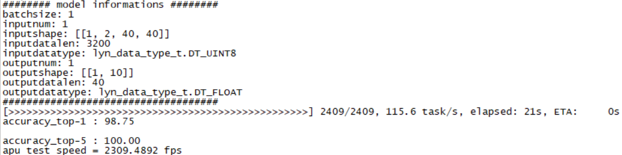
Figure: dvs-mnist data inference results#
Single machine multi-card deployment#
Design scheme for single machine multi-card#
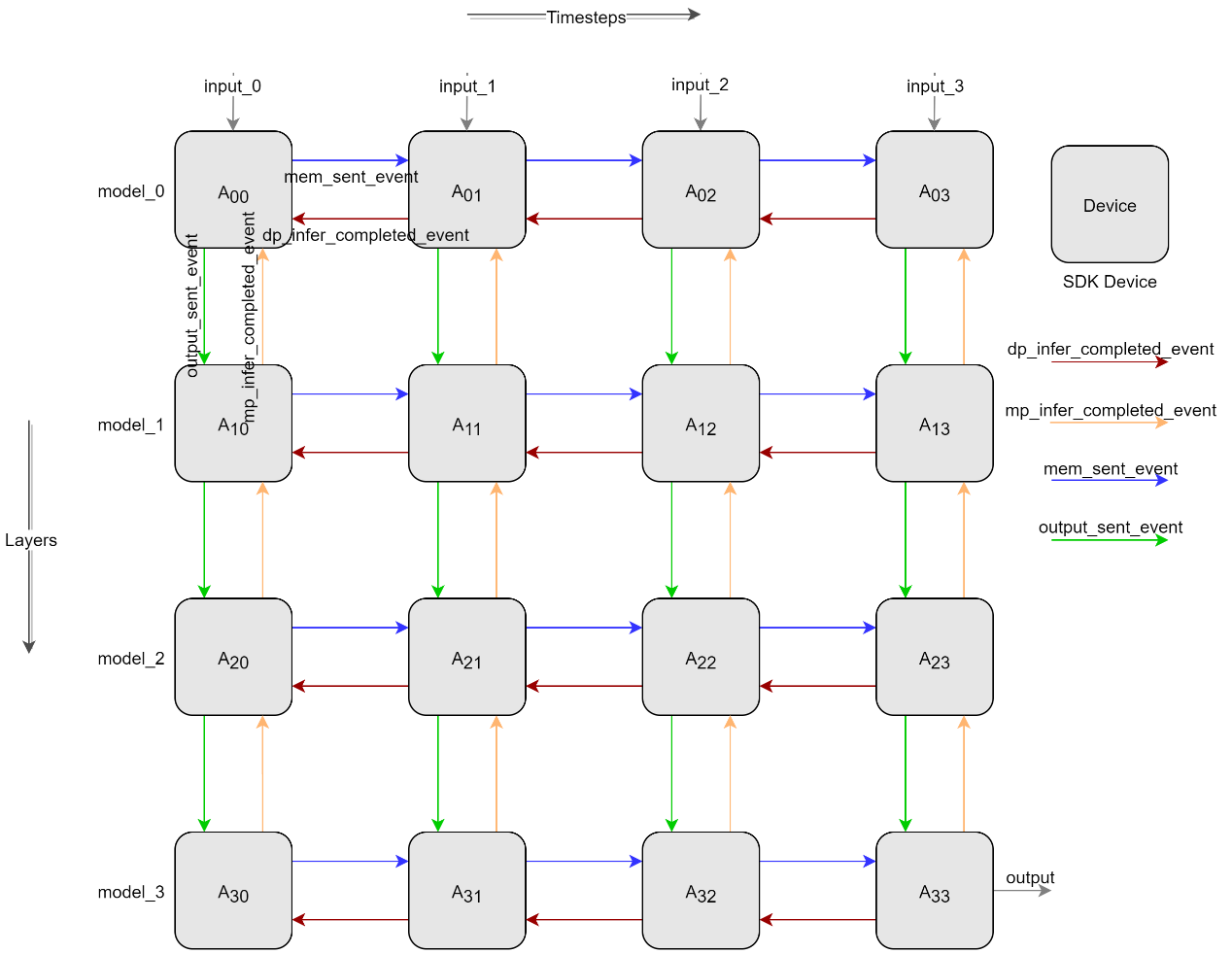
Figure: Pipeline parallel design diagram#
As shown in Figure: Pipeline parallel design diagram, horizontal denotes time-slicing, vertical denotes model-slicing, achieving multi-card pipeline parallel inference through spatiotemporal slicing. Data transfer and synchronization between Devices are done as shown by the arrows in Figure: Pipeline parallel design diagram. After horizontal A00 inference completion, confirm the event of receiving A01 inference complete (such as the red arrow), A00 sends the membrane potential to A01 and sends the membrane potential sent completion event (such as the red arrow), A01, after confirming the receipt of the membrane potential sent completion event, begins inference. After vertical A00 completes inference, it first confirms the receipt of the A10 inference complete event (such as the orange arrow), then sends the output to A10 and sends the output sent completion event (such as the green arrow), A10 begins inference using the A00 output as input after confirming receipt of the output sent completion event.
Single machine multi-card test results#
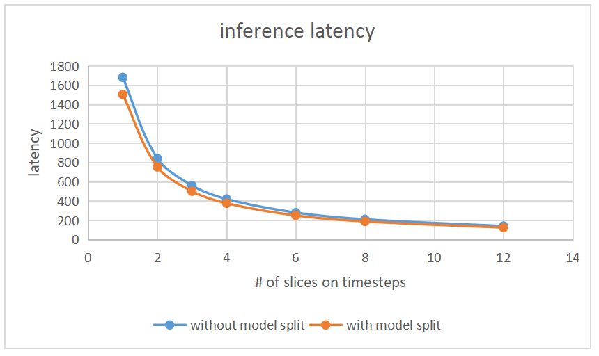
For situations where single-sample inference time is much greater than other overheads, frame rate increases linearly with the number of chips. The test results are shown in the following graphs.
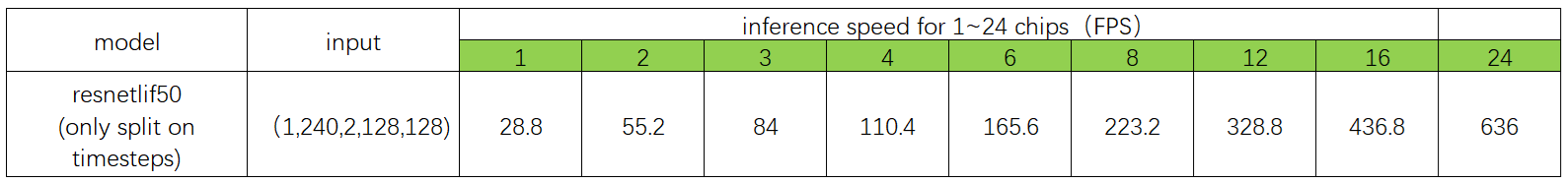
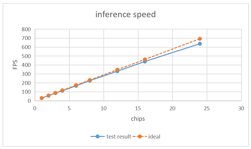
For the same number of chips, inference frame rate after spatiotemporal slicing is better than only time-frame slicing, as shown in the following graphs.
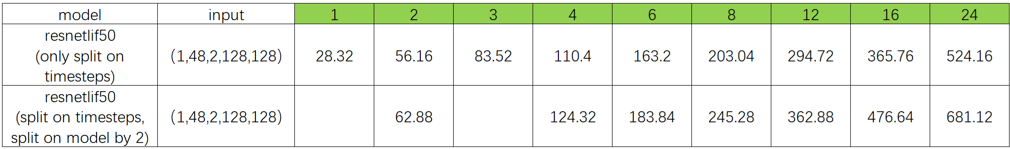
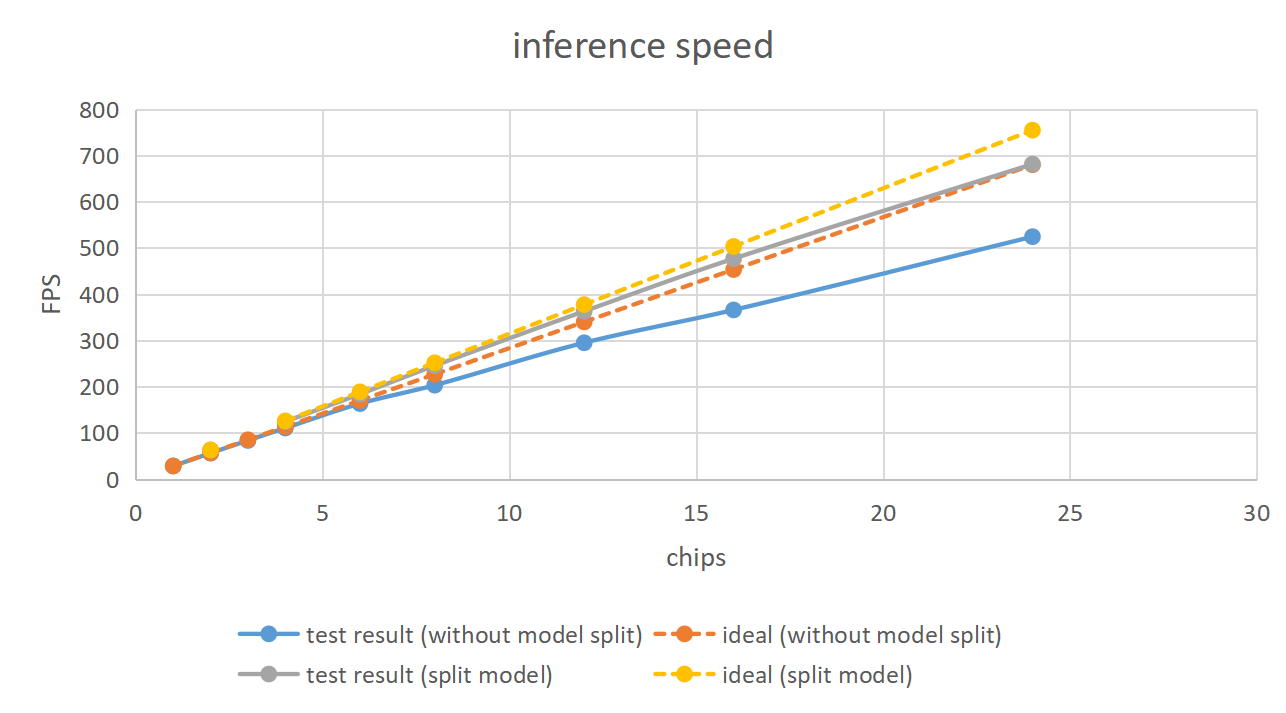
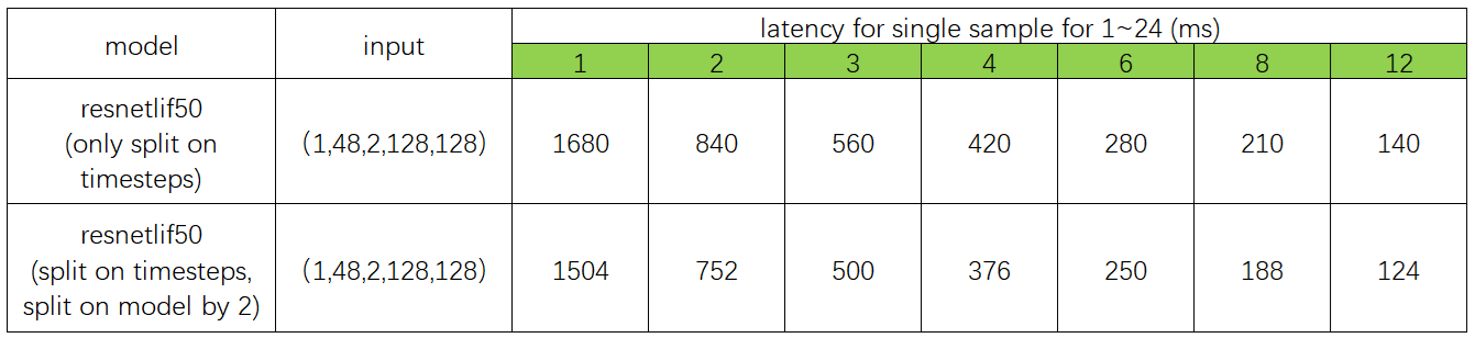
With the same input size, model slicing results in shorter inference time compared to single model inference. As shown above, model two with two chips after slicing has an inference speed greater than double the speed of a single chip with no slicing.
Source code and operation#
Code path: ./tools/
apuinfer_mutidevice.py: Single machine multi-card inference test script;
lyn_sdk_model_multidevice.py: Spatiotemporal slicing pipeline parallel SDK encapsulation class file;
complie_for_mp.py: Model slicing compilation script;
Compilation of Resentlif50 model slicing
Configuration file: resnetlif50-itout-b8x1-cifar10dvs_mp.py
models_compile_inputshape = [[1, 2, 128, 128], [1, 512, 16, 16]] # dim 0 represents the number of model slice; dim 1 represent the input shape of model slice;

model_0 = dict(
   type='ImageClassifier',
   backbone=dict(
      type='ResNetLifItout_MP',
      timestep=10,
      depth=50, nclass=10,
      down_t=[1, 'avg'],
      input_channels=2,
      noise=1e-5,
      soma_params='channel_share',
      cmode='spike',
      split=[0, 6] # layers included of model_0
   ),

   neck=None,
   head=dict(
      type='ClsHead',
      # loss=dict(type='CrossEntropyLoss', loss_weight=1.0),
      loss=dict(type='LabelSmoothLoss', label_smooth_val=0.1, loss_weight=1.0),
      topk=(1, 5),
      cal_acc=True
   )
)

model_1 = dict(
   type='ImageClassifier',
   backbone=dict(
      type='ResNetLifItout_MP',
      timestep=10,
      depth=50, nclass=10,
      down_t=[1, 'avg'],
      input_channels=2,
      noise=1e-5,
      soma_params='channel_share',
      cmode='spike',
      split=[6, 16] # layers included of model_1
   ),
   neck=None,
   head=dict(
      type='ClsHead',
      # loss=dict(type='CrossEntropyLoss', loss_weight=1.0),
      loss=dict(type='LabelSmoothLoss', label_smooth_val=0.1, loss_weight=1.0),
      topk=(1, 5),
      cal_acc=True
   )
)
Resnetlif50 Single Machine Multi-card Inference
Configuration file:
resnetlif50-itout-b8x1-cifar10dvs.py
# dim 0 represents the number of timesteps slices;
# dim 1 represents the number of model segments;
# value represents the device id;
# eg. lynxi_devices = [[0,1],[2,3],[4,5]], timesteps slices are 3, model segments are 2, device ids are 0,1,2,3,4,5.
# lynxi_devices = [[0],[1],[2],[3],[4],[5],[6],[7],[8],[9],[10],[11],[12],[13],[14],[15],[16],[17],[18],[19],[20],[21],[22],[23]]

lynxi_devices = [[0],[1]]
resnetlif50-itout-b8x1-cifar10dvs_mp.py
# dim 0 represents the number of timesteps slices;
# dim 1 represents the number of model segments;
# value represents the device id;
# eg. lynxi_devices = [[0,1],[2,3],[4,5]], timesteps slices are 3, model segments are 2, device ids are 0,1,2,3,4,5.
# lynxi_devices = [[0,1],[2,3],[4,5],[6,7],[8,9],[10,11],[12,13],[14,15],[16,17],[18,19],[20,21],[22,23]]

lynxi_devices = [[0,1]]
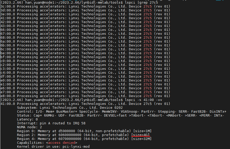
Test Environment
SDK version 1.11.0
apuinfer_mutidevice.py's default lyn_sdk_model_multidevice.via_p2p = Falseindicates P2P function is not used. If set to True, device support for P2P function is required. The red outlined section in the image below (size=4G) indicates device support for P2P function.